Most people think of Excel as merely a spreadsheet program, and with good reason—
Excel is a spreadsheet program. As a spreadsheet program, Excel is a powerful applicationthat provides a wide range of tools for the manipulation, analysis, and display
of data. Since its release it has become one of the most widely used spreadsheet application in the world.
How to use Excel
Step One: Plan Your Spreadsheet
- Before you begin entering data into a spreadsheet it is a good idea to do a bit of planning before you begin to type.
- Whenever possible, don't leave blank rows or columns when entering your data because it can make it difficult to usse a number of Excel's built in features such as graphing and functions.
- Enter your data in columns when possible - as seen in the image below.

Step Two: Enter Your Data into Your Spreadsheet
- Entering your data into a spreadsheet is always a three step process. These steps are:
Type your data into the cell.
Press the ENTER key on the keyboard or click on another cell with the mouse.
Step Three: AutoComplete
- Excel's AutoComplete feature is intended to simplify the task of entering data.
Step Four: Editing Cells
- Click on the cell, type over the existing entry, and press the ENTER key on the keyboard.
Parts of the Excel Screen

Active Cell:
The active cell is recognized by its black outline. Data is always entered into the active cell. Different cells can be made active by clicking on them with the mouse or by using the arrow keys on the keyboard.File Tab:
The File tab options are mostly related to file management such as opening new or existing worksheet files, saving, printing, and a new feature - saving and sending Excel files in PDF format.Formula Bar:
Located above the worksheet, this area displays the contents of the active cell. It can also be used for entering or editing data and formulas.Name Box:
Located next to the formula bar, the Name Box displays the cell reference or the name of the active cell.Column Letters:
Columns run vertically on a worksheet and each one is identified by a letter in the column header.Row Numbers:
Rows run horizontally in a worksheet and are identified by a number in the row header.Together a column letter and a row number create a cell reference. Each cell in the worksheet can be identified by this combination of letters and numbers such as A1, F456, or AA34.
Sheet Tabs:
By default there are three worksheets in an Excel file. The tab at the bottom of a worksheet tells you the name of the worksheet - such as Sheet1, Sheet2 etc.Switching between worksheets can be done by clicking on the tab of the sheet you wish to access. Renaming a worksheet or changing the tab color can make it easier to keep track of data in large spreadsheet files.Quick Access Toolbar:
This customizable toolbar allows you to add frequently used commands. Click on the down arrow at the end of the toolbar to display the toolbar's options.Ribbon:
The Ribbon is the strip of buttons and icons located above the work area. The Ribbon is organized into a series of tabs - such as File, Home, and Formulas.Uses of Microsoft Excel
1. Manage your finances with Excel
2. Create a personal or family budget
3. Create a calendar or schedule with Excel
4. Track your income and expenses
5. Manage your data records efficiently
Que es una Tabla Dinamica?
Una tabla dinámica combina y compara en forma rápida grandes volúmenes de datos. Permitiendo el análisis multidimensional de los datos al girar las filas y las columnas creando diferentes formas de visualizar reportes con los datos de origen. Llendo desde lo general a lo específico.
Las tablas dinámica solo sirven para resumir los datos según la consulta realizada, pero no permiten modelar dentro de la tabla. La opción posible sería tomar los datos de la Tabla Dinámica Excel con la función IMPORTAR DATOS DINAMICOS e incorporarlos a nuestro modelo Excel.
Crear una Tabla Dinamica:
1.) Sólo tienes que seguir estos 4 pasos para crear la tabla dinámica de Excel:
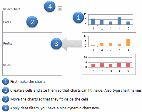
1. Prepare los gráficos: Hacer gráficos tantos como desee. Digamos que 3.
2. Configurar el área de gráficos dinámicos, donde se cargará: Basta con echar 3 celdas de una fila y ajustar el alto de fila y ancho de la columna de tal manera que los gráficos se pueden encajar dentro perfectamente. También, escriba los nombres de gráficos (1 para cada celda) en la célula. Digamos, las cartas que tiene son de costos, ventas y beneficios, sólo tienes que escribir estos nombres en las células.
3. Mover y colocar gráficos dentro de estas células: Esta debe ser simple.
4. Por último se aplican filtros de datos a la celda en la parte superior de las celdas 3. Seleccione una opción de filtro y sólo verá esa carta.
2.) El método de la tabla Una tabla dinámica combina y compara en forma rápida grandes volúmenes de datos. Permitiendo el análisis multidimensional de los datos al girar las filas y las columnas creando diferentes formas de visualizar reportes con los datos de origen. Llendo desde lo general a lo específico.
Las tablas dinámica solo sirven para resumir los datos según la consulta realizada, pero no permiten modelar dentro de la tabla. La opción posible sería tomar los datos de la Tabla Dinámica Excel con la función IMPORTAR DATOS DINAMICOS e incorporarlos a nuestro modelo Excel.
Crear una Tabla Dinamica:
1.) Sólo tienes que seguir estos 4 pasos para crear la tabla dinámica de Excel:
1. Prepare los gráficos: Hacer gráficos tantos como desee. Digamos que 3.
2. Configurar el área de gráficos dinámicos, donde se cargará: Basta con echar 3 celdas de una fila y ajustar el alto de fila y ancho de la columna de tal manera que los gráficos se pueden encajar dentro perfectamente. También, escriba los nombres de gráficos (1 para cada celda) en la célula. Digamos, las cartas que tiene son de costos, ventas y beneficios, sólo tienes que escribir estos nombres en las células.
3. Mover y colocar gráficos dentro de estas células: Esta debe ser simple.
4. Por último se aplican filtros de datos a la celda en la parte superior de las celdas 3. Seleccione una opción de filtro y sólo verá esa carta.
1.Haga clic en la pestaña Insertar.
2.In el grupo Tablas, haga clic en Tabla.
3.Excel mostrará el rango seleccionado, que puede cambiar. Si la tabla no tiene encabezados, asegúrese de desactivar la opción de tabla tiene encabezados.
4.Haga OK y Excel formatear el rango de datos como una tabla.


Cualquier gráfico que se basan en la mesa será dinámico. Para ilustrar, crear un gráfico de columnas rápida como sigue:
1.Seleccione la mesa.
2.Haga clic en la pestaña Insertar.
3.In el grupo Gráficos, seleccione la tabla de la primera columna en 2-D en la tabla desplegable.

Ahora bien, actualizar el gráfico mediante la adición de los valores de marzo y ver la tabla de actualización de forma automática.

No comments:
Post a Comment